Understanding shapes

import numpy as np
import matplotlib.pyplot as plt
from scipy import stats
from scipy.integrate import quad
from progressbar import progressbar as pbar
from rlxutils import subplots, copy_func
import pandas as pd
import seaborn as sns
import tensorflow as tf
import tensorflow_probability as tfp
tfd = tfp.distributions
tfb = tfp.bijectors

%matplotlib inline

2022-03-13 17:17:57.687505: W tensorflow/stream_executor/platform/default/dso_loader.cc:64] Could not load dynamic library 'libcudart.so.11.0'; dlerror: libcudart.so.11.0: cannot open shared object file: No such file or directory
2022-03-13 17:17:57.687542: I tensorflow/stream_executor/cuda/cudart_stub.cc:29] Ignore above cudart dlerror if you do not have a GPU set up on your machine.

observe that, besides batch_shape distributions have an associated event_shape, which in this case in empty, signalling that each distribution in the batch is a distribution of scalars.

d = tfd.Normal(loc=[-1,0], scale=1)
d

<tfp.distributions.Normal 'Normal' batch_shape=[2] event_shape=[] dtype=float32>

in general, picture yourself wanting to assigned different distributions to different data points in your datset.

Multivariate distributions

They have event_shape. For instance, for a multivariate normal distribution we must specify a covariance matrix. Observe that this cannot be done using uniquely the batch_size, since in general variables of a multivariate normal are not independant

# Initialize a single 3-variate Gaussian.
mu = [1., 2]
cov = [[ 0.36,  0.12],
       [ 0.12,  0.29]]

mvn = tfd.MultivariateNormalTriL(
    loc=mu,
    scale_tril=tf.linalg.cholesky(cov))

s = mvn.sample(10000)
s.shape

TensorShape([10000, 2])

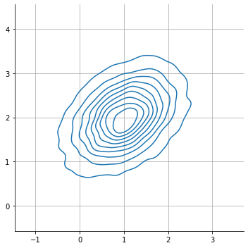
observe that dependance shows as a slanted plot

sns.displot( x = s[:,0], y = s[:,1], kind="kde", rug=False)
plt.axis("equal"); plt.grid();

observe that this implies an event_shape

mvn

<tfp.distributions.MultivariateNormalTriL 'MultivariateNormalTriL' batch_shape=[] event_shape=[2] dtype=float32>

Combining batch_shape and event_shape

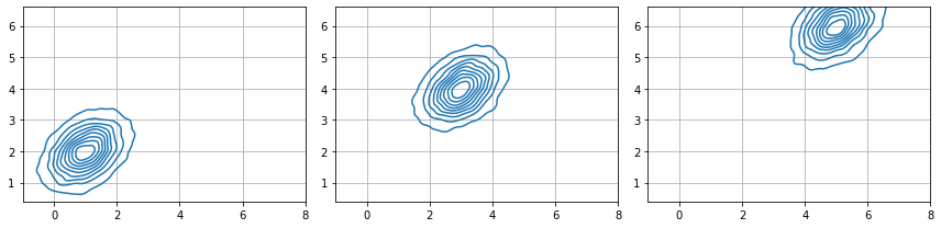
altogether both determine the sample sizes. Observe how we use broadcasting of the covariance matrix to have a batch of three multivariate distributions of two variables each. The three distributions have the same covariance matrix.

# Initialize a single 3-variate Gaussian.
mu = [[1., 2],[3,4], [5,6]]

cov = [[ 0.36,  0.12],
       [ 0.12,  0.29]]

mvn = tfd.MultivariateNormalTriL(
    loc=mu,
    scale_tril=tf.linalg.cholesky(cov)
)

mvn

<tfp.distributions.MultivariateNormalTriL 'MultivariateNormalTriL' batch_shape=[3] event_shape=[2] dtype=float32>

s = mvn.sample(10000)
s.shape

TensorShape([10000, 3, 2])

np.min(mu)

1.0

for ax,i in subplots(s.shape[1], usizex=4):    
    sns.kdeplot( x = s[:, i, 0], y = s[:, i, 1], ax=ax)
    plt.axis("equal"); plt.grid();
    plt.xlim(np.min(mu)-2, np.max(mu)+2)
    plt.ylim(np.min(mu)-4, np.max(mu)+4)
plt.tight_layout()

Making sense of shapes

In general, samples from a distribution will have the shape [sample_shape, batch_shape, event_shape]

• sample_shape is determined when you call the sample method of the distribution

• batch_shape is determined by the parameters of the distribution when you create it

• event_shape is detemrined by the nature of the multivariate distribution you use

This way:

• samples: are independant identically distributed

• batch components: are independant and NOT identically distributed

• event components: are NOT independant and NOT identiclly distributed

The following table might help make sense of this. It is based on this post and this post.

\[\begin{split} \begin{array}{|c|c|c|c|l|}\hline \textbf{sample shape}&\textbf{batch shape}&\textbf{event shape} & \textbf{distribution for samples} \\\hline \texttt{[2]}&\texttt{[]} &\texttt{[]} & X_0, X_1 \overset{iid}{\sim} \mathcal{N}(\mu, \sigma)&\text{one single variable distribution}\\\hline \texttt{[2]}&\texttt{[3]} &\texttt{[]} & X_{0,0}, X_{1,0} \overset{iid}{\sim} \mathcal{N}(\mu_0, \sigma_0)&\text{three single variable distributions}\\ &&& X_{0,1}, X_{1,1} \overset{iid}{\sim} \mathcal{N}(\mu_1, \sigma_1)\\ &&& X_{0,2}, X_{1,2} \overset{iid}{\sim} \mathcal{N}(\mu_2, \sigma_2)\\\hline \texttt{[2]}&\texttt{[]} &\texttt{[4]} & \mathbf{X}_0, \mathbf{X}_1 \overset{iid}{\sim} \mathcal{N}(\boldsymbol{\mu}, \boldsymbol{\sigma})\;\;\;\;\;\mathbf{X}_i\in\mathbb{R}^4&\text{one mutivariate distribution}\\\hline \texttt{[2]}&\texttt{[3]} &\texttt{[4]} & \mathbf{X}_{0,0}, \mathbf{X}_{1,0} \overset{iid}{\sim} \mathcal{N}(\boldsymbol{\mu}_0, \boldsymbol{\sigma}_0)\;\;\;\;\;\mathbf{X}_i\in\mathbb{R}^4&\text{three multivariate distributions}\\ &&& \mathbf{X}_{0,1}, \mathbf{X}_{1,1} \overset{iid}{\sim} \mathcal{N}(\boldsymbol{\mu}_1, \boldsymbol{\sigma}_1)\;\;\;\;\;\;\;\;\;\;\;\;\;\;\;\;\\ &&& \mathbf{X}_{0,2}, \mathbf{X}_{1,2} \overset{iid}{\sim} \mathcal{N}(\boldsymbol{\mu}_2, \boldsymbol{\sigma}_2)\;\;\;\;\;\;\;\;\;\;\;\;\;\;\;\;\\\hline \end{array} \end{split}\]

observe how we deal with each case in the code below

# batch_shape=[], event_shape=[]

d = tfd.Normal(loc=0, scale=1)
print (d)
print (d.sample(2).numpy())

tfp.distributions.Normal("Normal", batch_shape=[], event_shape=[], dtype=float32)
[ 0.75803363 -1.8501624 ]

# batch_shape=[3], event_shape=[]     implicitly with vector parameters

d = tfd.Normal(loc=[0,1,2], scale=1) # broadcasting on batch same for scale
print (d)
print (d.sample(2).numpy())

tfp.distributions.Normal("Normal", batch_shape=[3], event_shape=[], dtype=float32)
[[ 1.1833676  1.7853057  5.493244 ]
 [-1.2918025  2.284341   0.9959991]]

# batch_shape=[], event_shape=[4]        explicitly with a multivariate distribution

mu = np.random.random(4)*10-5
cov = np.random.random(size=(4,4))+.1    # will broadcast covariance matrix
cov = tf.linalg.cholesky(cov.dot(cov.T)) # ensures positive definite matrix

d = tfd.MultivariateNormalTriL(mu,cov)

print (d)
print (d.sample(2).numpy())

tfp.distributions.MultivariateNormalTriL("MultivariateNormalTriL", batch_shape=[], event_shape=[4], dtype=float64)
[[-4.94196295  4.54800186 -0.1223484  -2.39742009]
 [-6.22349008  2.51441253 -2.61423195 -3.71563902]]

# batch_shape=[3], event_shape=[4]

mu = np.random.random((3,4))*10-5

cov = np.random.random(size=(4,4))+.1    # will broadcast covariance matrix
cov = tf.linalg.cholesky(cov.dot(cov.T)) # ensures positive definite matrix

d = tfd.MultivariateNormalTriL(mu,cov)

print (d)
print (d.sample(2).numpy())

tfp.distributions.MultivariateNormalTriL("MultivariateNormalTriL", batch_shape=[3], event_shape=[4], dtype=float64)
[[[-5.1101803   0.8596026   3.06403109  2.1083541 ]
  [ 3.69974774 -3.93829998 -1.6255217   2.22765852]
  [ 3.32589202  2.69049452 -4.32719606  1.2584832 ]]

 [[-5.93515374  0.91773734  2.35591075  2.1539073 ]
  [ 6.17373777 -3.15403426 -0.98656476  2.23261819]
  [ 1.86732188  2.18168707 -5.64504685  1.01497814]]]

The Independent distribution object

Allows us to transfer dimensions from batch_shape to event_shape.

This might be useful when designing specific final distributions. Recall that batches are sets of distributions of the same family but with different parameters, so they are independant, whereas events belong to the same multivariate and maybe dependant.

# Initialize a single 3-variate Gaussian.
mu = np.random.random(size=(3,4,2)).astype(np.float32)

cov = [[ 0.36,  0.12],
       [ 0.12,  0.29]]

mvn = tfd.MultivariateNormalTriL(
    loc=mu,
    scale_tril=tf.linalg.cholesky(cov)
)

mvn

<tfp.distributions.MultivariateNormalTriL 'MultivariateNormalTriL' batch_shape=[3, 4] event_shape=[2] dtype=float32>

s = mvn.sample(100000)
s.shape

TensorShape([100000, 3, 4, 2])

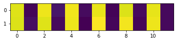
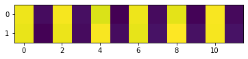
plt.imshow(np.mean(s, axis=0).reshape(2,-1))

<matplotlib.image.AxesImage at 0x7f42493bed90>

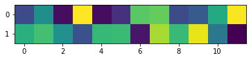
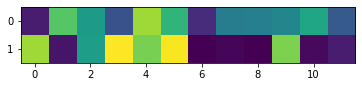
plt.imshow(np.std(s, axis=0).reshape(2,-1))

<matplotlib.image.AxesImage at 0x7f42492ca280>

redistribute dimensions

mi = tfd.Independent(mvn, reinterpreted_batch_ndims=1)
mi

<tfp.distributions.Independent 'IndependentMultivariateNormalTriL' batch_shape=[3] event_shape=[4, 2] dtype=float32>

observe that samples have the same shape and individual distributions

s = mi.sample(100000)
s.shape

TensorShape([100000, 3, 4, 2])

plt.imshow(np.mean(s, axis=0).reshape(2,-1))

<matplotlib.image.AxesImage at 0x7f95845115e0>

plt.imshow(np.std(s, axis=0).reshape(2,-1))

<matplotlib.image.AxesImage at 0x7f9584442340>